Custom Latitude Distributions

This notebook shows how to define a custom starspot latitude distribution by subclassing LatitudeDistributionFunction and how it propagates through the spotgp pipeline.

Two roles of the latitude distribution:

Component	Role
AnalyticKernel	PDF weights the latitude integral \(\int p(\phi)\,K(\phi,\tau)\,d\phi\)
LightcurveModel.from_spot_model	lat_range sets the uniform sampling bounds for spot placement

Sections

1. Default uniform distribution

2. Equatorial band — narrow lat_range

3. Gaussian-weighted distribution — custom PDF over latitude

4. Polar band — spots at high latitudes

5. Kernel and lightcurve comparison across all distributions

import sys
sys.path.append("../..")

import numpy as np
import matplotlib.pyplot as plt
import jax.numpy as jnp

from spotgp import (
    LatitudeDistributionFunction,
    TrapezoidSymmetricEnvelope,
    VisibilityFunction,
    SpotEvolutionModel,
    LightcurveModel,
    AnalyticKernel,
)

label_fs = 18
np.random.seed(42)

# Shared model components reused throughout
_envelope   = TrapezoidSymmetricEnvelope(lspot=15.0, tau_spot=5.0)
_visibility = VisibilityFunction(peq=10.0, kappa=0.3, inc=np.pi / 3)

---

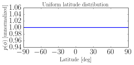
1. Default uniform distribution

When no latitude_distribution is supplied to SpotEvolutionModel, a LatitudeDistributionFunction() is used — uniform over \([-\pi/2,\, \pi/2]\) (all latitudes with equal weight).

lat_uniform = LatitudeDistributionFunction()
print(lat_uniform)
print("lat_range :", lat_uniform.lat_range)
print("p(0)      :", lat_uniform(0.0))
print("p(pi/4)   :", lat_uniform(np.pi / 4))

model_uniform = SpotEvolutionModel(
    envelope=_envelope,
    visibility=_visibility,
    sigma_k=0.01,
    # latitude_distribution defaults to LatitudeDistributionFunction()
)

LatitudeDistributionFunction(lat_range=[-1.571, 1.571])
lat_range : (-1.5707963267948966, 1.5707963267948966)
p(0)      : 1.0
p(pi/4)   : 1.0

phi = np.linspace(-np.pi / 2, np.pi / 2, 300)
pdf_vals = np.array([lat_uniform(p) for p in phi])

fig, ax = plt.subplots(figsize=(6, 3))
ax.plot(np.rad2deg(phi), pdf_vals, lw=2)
ax.set_xlabel("Latitude [deg]", fontsize=label_fs)
ax.set_ylabel(r"$p(\phi)$ [unnormalized]", fontsize=label_fs)
ax.set_title("Uniform latitude distribution", fontsize=label_fs)
ax.set_xlim(-90, 90)
ax.set_xticks(np.arange(-90, 91, 30))
fig.tight_layout()
plt.show()

---

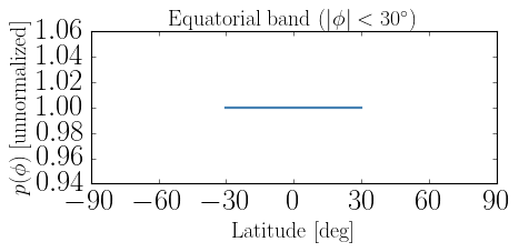
2. Equatorial band

Restrict spots to low latitudes by overriding lat_range. The PDF itself remains uniform within the narrower range.

class EquatorialBand(LatitudeDistributionFunction):
    """Uniform distribution confined to |phi| < max_lat."""

    def __init__(self, max_lat_deg: float = 30.0):
        self._max_lat = float(np.deg2rad(max_lat_deg))

    @property
    def lat_range(self) -> tuple:
        return (-self._max_lat, self._max_lat)

    def __call__(self, phi: float) -> float:
        return 1.0


lat_equatorial = EquatorialBand(max_lat_deg=30.0)
print(lat_equatorial)
print("lat_range :", tuple(np.rad2deg(lat_equatorial.lat_range).round(1)), "deg")

model_equatorial = SpotEvolutionModel(
    envelope=_envelope,
    visibility=_visibility,
    sigma_k=0.01,
    latitude_distribution=lat_equatorial,
)

EquatorialBand(lat_range=[-0.524, 0.524])
lat_range : (np.float64(-30.0), np.float64(30.0)) deg

phi_eq  = np.linspace(*lat_equatorial.lat_range, 300)
pdf_eq  = np.array([lat_equatorial(p) for p in phi_eq])

fig, ax = plt.subplots(figsize=(6, 3))
ax.plot(np.rad2deg(phi_eq), pdf_eq, lw=2, color="steelblue")
ax.set_xlabel("Latitude [deg]", fontsize=label_fs)
ax.set_ylabel(r"$p(\phi)$ [unnormalized]", fontsize=label_fs)
ax.set_title(r"Equatorial band ($|\phi| < 30^\circ$)", fontsize=label_fs)
ax.set_xlim(-90, 90)
ax.set_xticks(np.arange(-90, 91, 30))
fig.tight_layout()
plt.show()

---

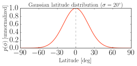
3. Gaussian-weighted distribution

A Gaussian PDF smoothly down-weights high latitudes rather than cutting them off sharply. Both lat_range and __call__ are overridden.

class GaussianLatitude(LatitudeDistributionFunction):
    """
    Gaussian PDF centred at `center` with standard deviation `sigma`.

    Spots can emerge anywhere within ±3σ of the center, but are weighted
    toward the center of the distribution.
    """

    def __init__(self, sigma_deg: float = 20.0, center_deg: float = 0.0):
        self._sigma  = float(np.deg2rad(sigma_deg))
        self._center = float(np.deg2rad(center_deg))

    @property
    def lat_range(self) -> tuple:
        return (self._center - 3 * self._sigma,
                self._center + 3 * self._sigma)

    def __call__(self, phi: float) -> float:
        return float(np.exp(-0.5 * ((phi - self._center) / self._sigma) ** 2))


lat_gauss = GaussianLatitude(sigma_deg=20.0)
print(lat_gauss)
print("lat_range :", tuple(np.rad2deg(lat_gauss.lat_range).round(1)), "deg")
print("p(0)      :", lat_gauss(0.0))
print("p(30 deg) :", lat_gauss(np.deg2rad(30.0)))

model_gauss = SpotEvolutionModel(
    envelope=_envelope,
    visibility=_visibility,
    sigma_k=0.01,
    latitude_distribution=lat_gauss,
)

GaussianLatitude(lat_range=[-1.047, 1.047])
lat_range : (np.float64(-60.0), np.float64(60.0)) deg
p(0)      : 1.0
p(30 deg) : 0.32465246735834974

phi_g   = np.linspace(-np.pi / 2, np.pi / 2, 300)
pdf_g   = np.array([lat_gauss(p) for p in phi_g])

fig, ax = plt.subplots(figsize=(6, 3))
ax.plot(np.rad2deg(phi_g), pdf_g, lw=2, color="tomato")
ax.axvline(0, color="k", lw=0.8, ls="--", alpha=0.5)
ax.set_xlabel("Latitude [deg]", fontsize=label_fs)
ax.set_ylabel(r"$p(\phi)$ [unnormalized]", fontsize=label_fs)
ax.set_title(r"Gaussian latitude distribution ($\sigma = 20^\circ$)", fontsize=label_fs)
ax.set_xlim(-90, 90)
ax.set_xticks(np.arange(-90, 91, 30))
fig.tight_layout()
plt.show()

---

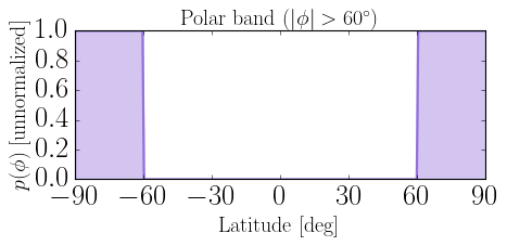
4. Polar band

Spots confined to high latitudes (like solar polar faculae). Implemented as two symmetric bands, one at each pole.

class PolarBand(LatitudeDistributionFunction):
    """
    Two symmetric bands near the poles: |phi| in [min_lat, pi/2].
    """

    def __init__(self, min_lat_deg: float = 60.0):
        self._min_lat = float(np.deg2rad(min_lat_deg))

    @property
    def lat_range(self) -> tuple:
        # Full range so spots can land at either pole
        return (-np.pi / 2, np.pi / 2)

    def __call__(self, phi: float) -> float:
        # Non-zero weight only at high latitudes
        return 1.0 if abs(phi) >= self._min_lat else 0.0


lat_polar = PolarBand(min_lat_deg=60.0)
print(lat_polar)
print("p(0)      :", lat_polar(0.0))
print("p(70 deg) :", lat_polar(np.deg2rad(70.0)))

model_polar = SpotEvolutionModel(
    envelope=_envelope,
    visibility=_visibility,
    sigma_k=0.01,
    latitude_distribution=lat_polar,
)

PolarBand(lat_range=[-1.571, 1.571])
p(0)      : 0.0
p(70 deg) : 1.0

phi_p   = np.linspace(-np.pi / 2, np.pi / 2, 300)
pdf_p   = np.array([lat_polar(p) for p in phi_p])

fig, ax = plt.subplots(figsize=(6, 3))
ax.fill_between(np.rad2deg(phi_p), pdf_p, alpha=0.4, color="mediumpurple")
ax.plot(np.rad2deg(phi_p), pdf_p, lw=2, color="mediumpurple")
ax.set_xlabel("Latitude [deg]", fontsize=label_fs)
ax.set_ylabel(r"$p(\phi)$ [unnormalized]", fontsize=label_fs)
ax.set_title(r"Polar band ($|\phi| > 60^\circ$)", fontsize=label_fs)
ax.set_xlim(-90, 90)
ax.set_xticks(np.arange(-90, 91, 30))
fig.tight_layout()
plt.show()

---

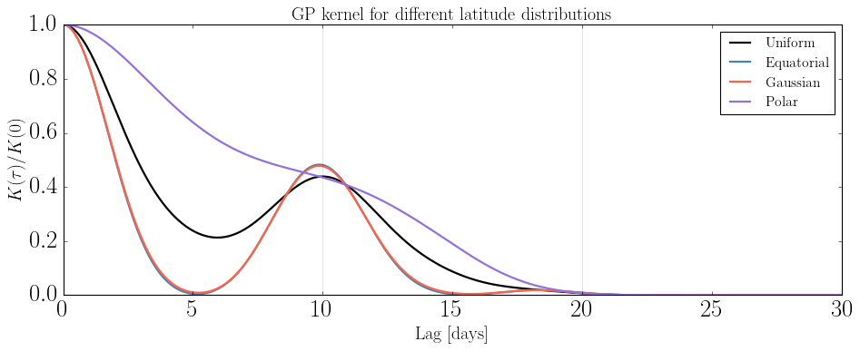
5. Kernel and lightcurve comparison

5a. GP kernel shapes

The latitude distribution modifies which latitudes contribute to the kernel integral. Spots at different latitudes rotate at different speeds (differential rotation), so the kernel shape — and in particular how quickly the periodic signal dephases — depends on the latitude distribution.

models = {
    "Uniform":    model_uniform,
    "Equatorial": model_equatorial,
    "Gaussian":   model_gauss,
    "Polar":      model_polar,
}
colors = {
    "Uniform":    "k",
    "Equatorial": "steelblue",
    "Gaussian":   "tomato",
    "Polar":      "mediumpurple",
}

lag = np.linspace(0, 3 * _visibility.peq, 400)
kernels = {}
for name, mdl in models.items():
    ak = AnalyticKernel(mdl)
    K  = ak.kernel(lag)
    kernels[name] = K

fig, ax = plt.subplots(figsize=(12, 5))
for name, K in kernels.items():
    ax.plot(lag, K / K[0], label=name, color=colors[name], lw=2)
for n in range(1, int(lag[-1] / _visibility.peq) + 1):
    ax.axvline(n * _visibility.peq, color="k", alpha=0.1, lw=1)
ax.set_xlabel("Lag [days]", fontsize=label_fs)
ax.set_ylabel(r"$K(\tau) / K(0)$", fontsize=label_fs)
ax.set_title("GP kernel for different latitude distributions", fontsize=label_fs)
ax.legend(fontsize=14)
ax.set_xlim(lag[0], lag[-1])
fig.tight_layout()
plt.show()

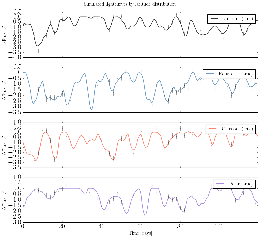
5b. Lightcurve comparison

LightcurveModel.from_spot_model uses lat_range from the latitude distribution to set the bounds for uniform spot placement. The PDF shape (if non-uniform) affects only the kernel integration in AnalyticKernel; the forward simulation always samples uniformly within lat_range. For a non-uniform forward simulation you would need to implement rejection sampling from the PDF.

fig, axes = plt.subplots(len(models), 1, figsize=(13, 3 * len(models)),
                         sharex=True)

for ax, (name, mdl) in zip(axes, models.items()):
    lc = LightcurveModel.from_spot_model(
        mdl, nspot=30, tsim=120, tsamp=0.5,
    )
    sigma_n  = 0.3 * np.std(lc.flux)
    flux_obs = lc.flux + np.random.normal(0, sigma_n, lc.flux.shape)

    ax.plot(lc.t, (lc.flux - 1) * 100, color=colors[name], lw=2,
            alpha=0.8, label=f"{name} (true)")
    ax.errorbar(lc.t[::4], (flux_obs[::4] - 1) * 100,
                yerr=sigma_n * 100,
                fmt=".k", ms=3, capsize=0, alpha=0.4)
    ax.set_ylabel(r"$\Delta$Flux [\%]", fontsize=label_fs)
    ax.set_xlim(lc.t[0], lc.t[-1])
    ax.legend(fontsize=label_fs, loc="upper right")

axes[-1].set_xlabel("Time [days]", fontsize=label_fs)
fig.suptitle("Simulated lightcurves by latitude distribution", fontsize=label_fs)
fig.tight_layout()
plt.show()

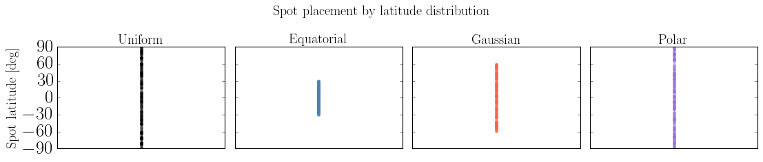
5c. Spot latitude placement

The scatter plot below shows which latitudes are drawn for each model. Latitudes outside lat_range are never placed; within lat_range the sampling is always uniform (regardless of the PDF shape).

np.random.seed(7)
nspot = 200
fig, axes = plt.subplots(1, len(models), figsize=(14, 3), sharey=True)

for ax, (name, mdl) in zip(axes, models.items()):
    lc = LightcurveModel.from_spot_model(
        mdl, nspot=nspot, tsim=200, tsamp=1.0,
    )
    lats_deg = np.rad2deg(lc.lat)
    ax.scatter(np.zeros(nspot), lats_deg, alpha=0.3, s=10, color=colors[name])
    ax.set_title(name, fontsize=label_fs)
    ax.set_xlim(-0.5, 0.5)
    ax.set_ylim(-90, 90)
    ax.set_yticks(np.arange(-90, 91, 30))
    ax.set_xticks([])

axes[0].set_ylabel("Spot latitude [deg]", fontsize=label_fs)
fig.suptitle("Spot placement by latitude distribution", fontsize=label_fs)
fig.tight_layout()
plt.show()