Probabilistic Graphical Model Visualization

A probabilistic graphical model (PGM) is a diagram that shows the dependencies between all variables in a statistical model — which parameters are free, which quantities are observed, and how they relate through deterministic functions and probability distributions.

spotgp can generate PGMs automatically from a configured GPSolver or MultiBandGPSolver. The diagram adapts to the model configuration: envelope type, whether noise is a free parameter, single- vs. multi-band mode, etc.

Diagram conventions:

Symbol	Meaning
Open circle	Latent (free) parameter
Shaded circle	Observed variable
Small dot	Fixed / known input
Ellipse	Deterministic function of parents
Rectangle (plate)	Repeated structure
Arrow	Dependency

import numpy as np
import matplotlib.pyplot as plt

from spotgp import (
    GPSolver,
    TrapezoidSymmetricEnvelope,
    TrapezoidAsymmetricEnvelope,
    VisibilityFunction,
    SpotEvolutionModel,
    PGModelVis,
)
from spotgp.multiband import MultiBandData, MultiBandGPSolver

np.random.seed(42)

# Shared synthetic data for all examples
x = np.linspace(0, 30, 200)
y = 1.0 + 0.01 * np.sin(2 * np.pi * x / 5.0) + 0.001 * np.random.randn(len(x))
yerr = 0.001 * np.ones_like(x)

---

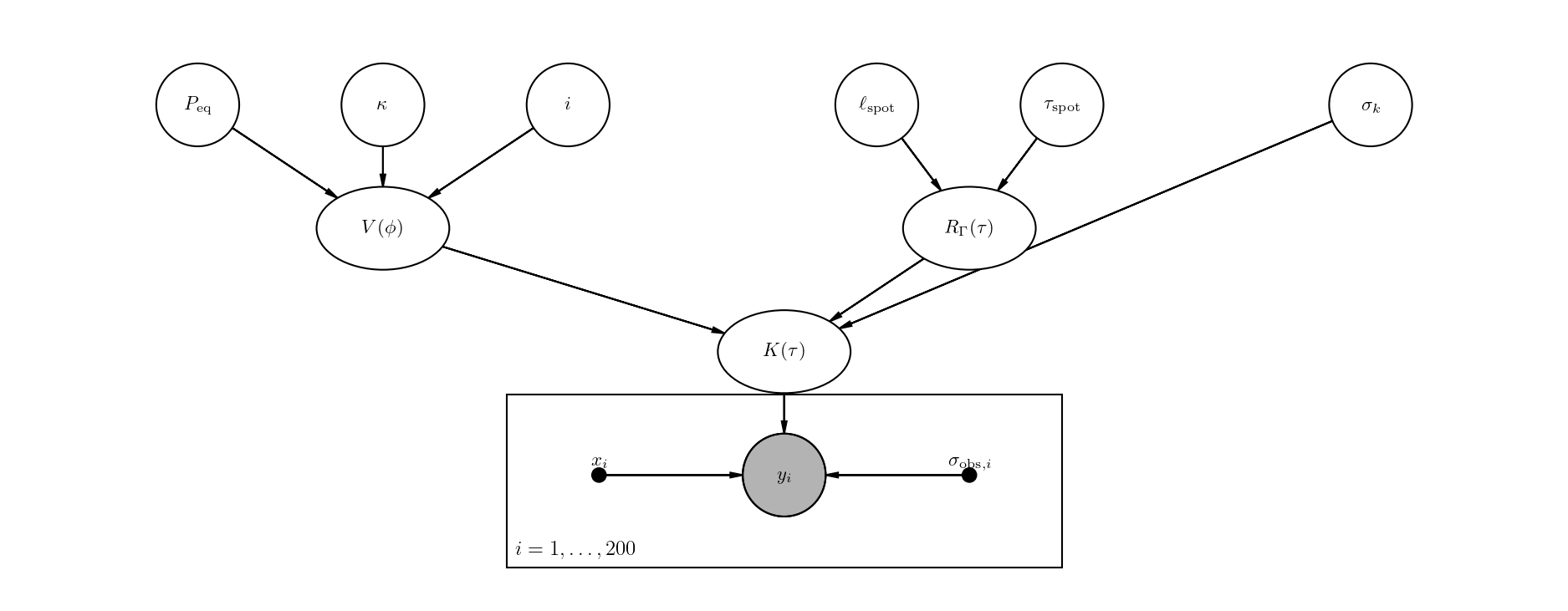
1. Default single-band GP

The simplest case: a symmetric trapezoid envelope with six free kernel parameters (\(P_{\rm eq}\), \(\kappa\), \(i\), \(\ell_{\rm spot}\), \(\tau_{\rm spot}\), \(\sigma_k\)) and no free noise term.

The PGM shows how the rotation parameters feed into the visibility function \(V(\phi)\), the envelope parameters feed into \(R_\Gamma(\tau)\), and both combine with \(\sigma_k\) to form the kernel \(K(\tau)\) that generates the observed flux \(y_i\).

hparam = dict(peq=5.0, kappa=0.3, inc=1.2, lspot=5.0, tau_spot=2.0, sigma_k=0.01)

gp = GPSolver(x, y, yerr, hparam)
fig = gp.plot_pgm()
plt.show()

Banded Cholesky: bandwidth=199, N=200, sparsity=0.0%

---

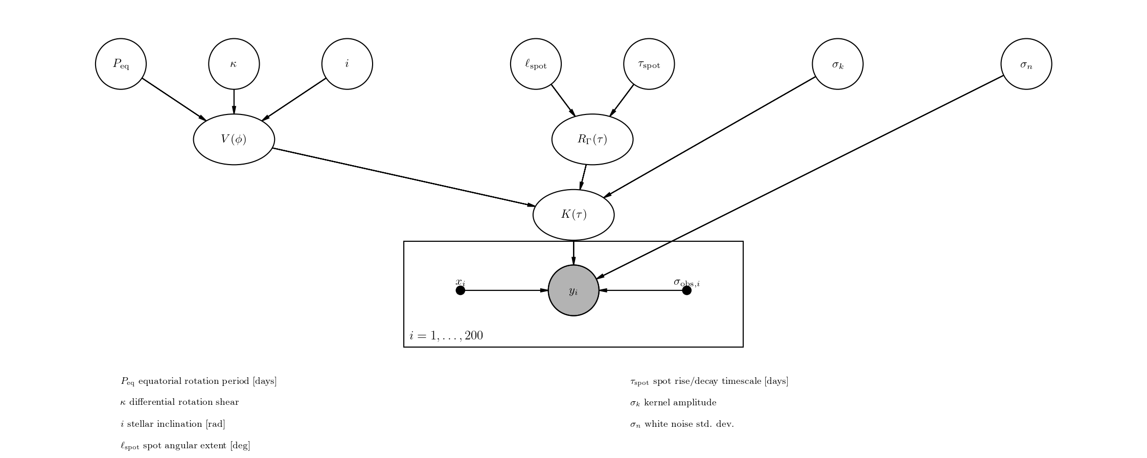
2. Adding white noise as a free parameter

Setting fit_sigma_n=True adds \(\sigma_n\) as a seventh free parameter. In the PGM it connects directly to \(y_i\) (not through the kernel), reflecting that white noise is added independently to each observation.

gp_noise = GPSolver(x, y, yerr, hparam, fit_sigma_n=True)

print("Free parameters:", gp_noise.param_keys)

fig = gp_noise.plot_pgm(show_legend=True)
plt.show()

Banded Cholesky: bandwidth=199, N=200, sparsity=0.0%

Free parameters: ('peq', 'kappa', 'inc', 'lspot', 'tau_spot', 'sigma_k', 'sigma_n')

---

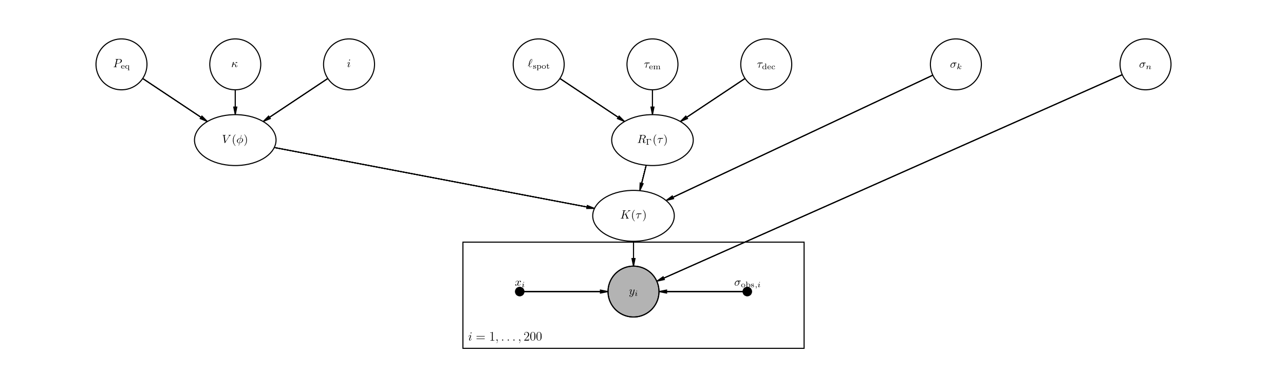
3. Asymmetric envelope

Switching to a TrapezoidAsymmetricEnvelope replaces \(\tau_{\rm spot}\) with separate emergence and decay timescales (\(\tau_{\rm em}\), \(\tau_{\rm dec}\)). The PGM automatically shows three parameters feeding into \(R_\Gamma(\tau)\) instead of two.

envelope_asym = TrapezoidAsymmetricEnvelope(lspot=5.0, tau_em=1.0, tau_dec=3.0)
visibility = VisibilityFunction(peq=5.0, kappa=0.3, inc=1.2)
model_asym = SpotEvolutionModel(
    envelope=envelope_asym, visibility=visibility, sigma_k=0.01,
)

gp_asym = GPSolver(x, y, yerr, model_asym, fit_sigma_n=True)

print("Free parameters:", gp_asym.param_keys)

fig = gp_asym.plot_pgm()
plt.show()

Banded Cholesky: bandwidth=199, N=200, sparsity=0.0%

Free parameters: ('peq', 'kappa', 'inc', 'lspot', 'tau_em', 'tau_dec', 'sigma_k', 'sigma_n')

---

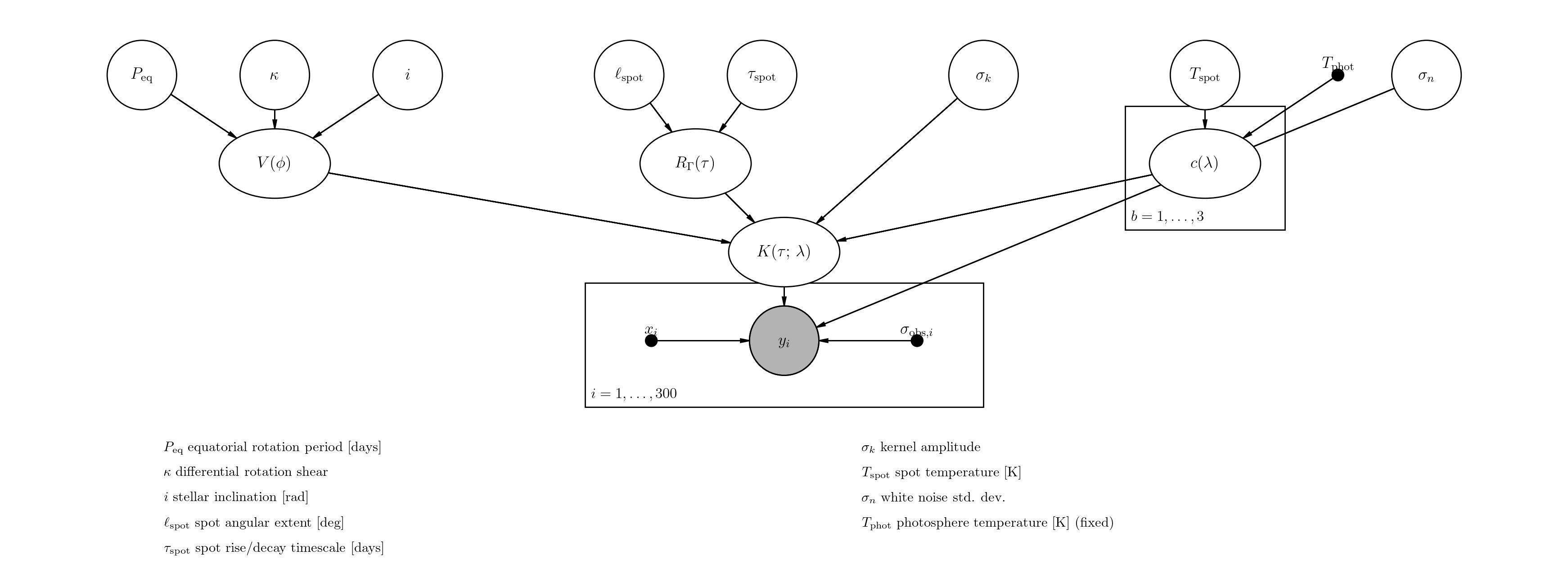
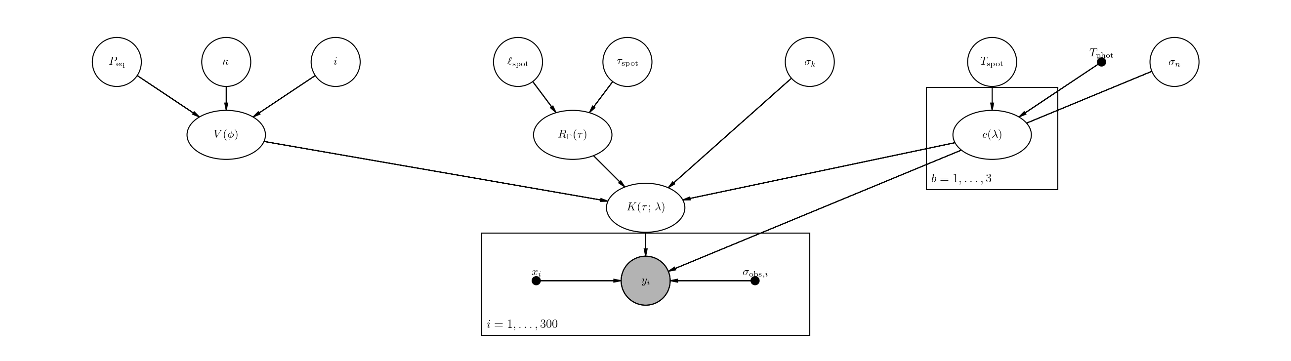
4. Multi-band GP

MultiBandGPSolver adds the spot temperature \(T_{\rm spot}\) as a free parameter and introduces the wavelength-dependent contrast factor \(c(\lambda) = 1 - B_\lambda(T_{\rm spot}) / B_\lambda(T_{\rm phot})\).

The PGM shows:

• \(T_{\rm spot}\) (free, open circle) and \(T_{\rm phot}\) (fixed, small dot) feeding into \(c(\lambda)\)

• \(c(\lambda)\) inside a band plate (\(b = 1, \ldots, B\)), since there is one contrast value per photometric band

• The kernel is labeled \(K(\tau;\,\lambda)\) to indicate its wavelength dependence

# Build three-band synthetic data
bands = {}
for name, lam in [("g", 4770.0), ("r", 6231.0), ("i", 7625.0)]:
    xb = np.sort(np.random.uniform(0, 30, 100))
    yb = 1.0 + 0.005 * np.sin(2 * np.pi * xb / 5.0) + 0.001 * np.random.randn(100)
    bands[name] = {"x": xb, "y": yb, "yerr": 0.001 * np.ones(100), "wavelength": lam}

data = MultiBandData(bands)

gp_mb = MultiBandGPSolver(
    data,
    hparam,
    T_phot=5800.0,
    T_spot_init=4500.0,
    fit_sigma_n=True,
)

print("Free parameters:", gp_mb.param_keys)
print(f"Bands: {data.band_names}  (N = {data.N} total observations)")

fig = gp_mb.plot_pgm()
plt.show()

MultiBand banded Cholesky: bandwidth=299, N=300, n_bands=3, sparsity=0.0%
Free parameters: ('peq', 'kappa', 'inc', 'lspot', 'tau_spot', 'sigma_k', 'T_spot', 'sigma_n')
Bands: ['g', 'r', 'i']  (N = 300 total observations)

---

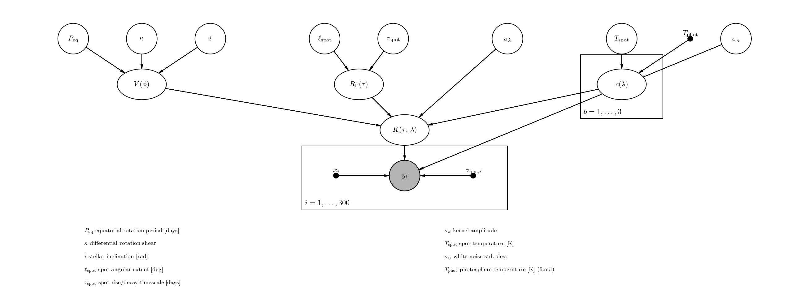
5. Parameter legend

Pass show_legend=True to add a key below the diagram that maps each LaTeX symbol to a descriptive name. This is useful for presentations or papers where readers may not be familiar with the notation.

fig = gp_noise.plot_pgm(show_legend=True)
plt.show()

The legend adapts to the model — here is the multi-band case, which includes \(T_{\rm spot}\) and marks \(T_{\rm phot}\) as fixed.

fig = gp_mb.plot_pgm(show_legend=True)
plt.show()

---

6. Using PGModelVis directly

You can also create a PGModelVis object directly to inspect the detected parameter groups or to customize dpi, node_scale, and font_size.

vis = PGModelVis(gp_mb)

print("Rotation params: ", vis.rotation_params)
print("Envelope params: ", vis.envelope_params)
print("Amplitude params:", vis.amplitude_params)
print("Multiband params:", vis.multiband_params)
print("Noise params:    ", vis.noise_params)

fig = vis.render(dpi=200, node_scale=1.4, font_size=13, show_legend=True)
plt.show()

Rotation params:  ['peq', 'kappa', 'inc']
Envelope params:  ['lspot', 'tau_spot']
Amplitude params: ['sigma_k']
Multiband params: ['T_spot']
Noise params:     ['sigma_n']