Custom Visibility Functions#
The base VisibilityFunction uses a small-spot approximation where the projected area of a spot simplifies to
which allows closed-form Fourier coefficients \(c_n(I, \Phi)\). This is accurate when the spot angular radius \(\alpha_{\max} \lesssim 6°\) (typical for Sun-like stars), but breaks down for large spots.
This notebook demonstrates how to subclass VisibilityFunction to implement the exact piecewise projected area from Eq. 5 of Birky et al., and finds where the small-spot approximation begins to diverge.
import sys
sys.path.append("../..")

import numpy as np
import jax.numpy as jnp
import matplotlib.pyplot as plt

from spotgp import (
    VisibilityFunction,
    FullGeometryVisibilityFunction,
    TrapezoidSymmetricEnvelope,
    SpotEvolutionModel,
    AnalyticKernel,
)

plt.rcParams.update({
    "font.size":        16,   # base font size
    "axes.titlesize":   20,   # axes title
    "axes.labelsize":   18,   # x/y axis labels
    "xtick.labelsize":  14,   # x tick labels
    "ytick.labelsize":  14,   # y tick labels
    "legend.fontsize":  14,
    "figure.titlesize": 22,   # suptitle
    "axes.formatter.useoffset": False,  # disable scientific notation offset
})
1. The exact projected area#
The full equation
The projected area of a circular spot with angular radius \(\alpha\) at angle \(\beta\) from the line of sight has three geometric regimes:
where \(\beta_k\) is the angle between the spot normal and the line of sight:
The three cases correspond to:
Fully visible: the entire spot disk is on the near hemisphere
Partially visible: the spot straddles the stellar limb
Hidden: the spot is on the far side
2. Implementing a custom VisibilityFunction#
To create a custom visibility function, subclass VisibilityFunction and override cn_squared(). The key methods to implement are:
Method |
Purpose |
|---|---|
|
Compute projected area for given spot size and angle |
|
Angle between spot normal and line of sight |
|
Squared Fourier coefficients (override base class) |
Here is the implementation of FullGeometryVisibilityFunction (which can be found in visibility.py)
class FullGeometryVisibilityFunction(VisibilityFunction):
    """
    Exact projected spot area using the full piecewise geometry,
    without the small-spot approximation.
    """

    def __init__(self, peq, kappa, inc, alpha_ref=0.1, n_lon=512):
        super().__init__(peq=peq, kappa=kappa, inc=inc)
        self.alpha_ref = float(alpha_ref)
        self.n_lon = int(n_lon)

    @staticmethod
    def projected_area(alpha, beta):
        """Exact projected area A(alpha, beta) — Eq. 5."""
        alpha = jnp.asarray(alpha)
        beta = jnp.asarray(beta)

        cos_a, sin_a = jnp.cos(alpha), jnp.sin(alpha)
        cos_b, sin_b = jnp.cos(beta), jnp.sin(beta)

        eps = 1e-30
        csc_b = 1.0 / (sin_b + eps)
        cot_b = cos_b / (sin_b + eps)
        cot_a = cos_a / (sin_a + eps)

        # Case 1: fully visible
        A_full = jnp.pi * sin_a**2 * cos_b

        # Case 2: partially visible
        arg1 = jnp.clip(cos_a * csc_b, -1.0, 1.0)
        arg2 = jnp.clip(-cot_a * cot_b, -1.0, 1.0)
        sqrt_arg = jnp.clip(1.0 - cos_a**2 * csc_b**2, 0.0, None)

        A_partial = (jnp.arccos(arg1)
                     + cos_b * sin_a**2 * jnp.arccos(arg2)
                     - cos_a * sin_b * jnp.sqrt(sqrt_arg))

        # Select case
        half_pi = jnp.pi / 2.0
        A = jnp.where(beta < half_pi - alpha, A_full,
                      jnp.where(beta > half_pi + alpha, 0.0, A_partial))
        return jnp.where(alpha > 1e-15, A, 0.0)

    def cos_beta(self, phi, longitude):
        """cos(beta) from Eq. 6."""
        return (jnp.cos(self.inc) * jnp.sin(phi)
                + jnp.sin(self.inc) * jnp.cos(phi) * jnp.cos(longitude))

    def cn_squared(self, phi, n_harmonics=3):
        """Fourier coefficients via numerical DFT of exact area profile."""
        lon = jnp.linspace(0, 2 * jnp.pi, self.n_lon, endpoint=False)
        cos_b = self.cos_beta(phi, lon)
        beta = jnp.arccos(jnp.clip(cos_b, -1.0, 1.0))
        A = self.projected_area(self.alpha_ref, beta)

        norm = jnp.pi * jnp.sin(self.alpha_ref)**2
        A_norm = A / jnp.where(norm > 1e-30, norm, 1.0)

        fft_coeffs = jnp.fft.rfft(A_norm) / len(A_norm)
        cn = jnp.abs(fft_coeffs[:n_harmonics + 1])
        return cn**2
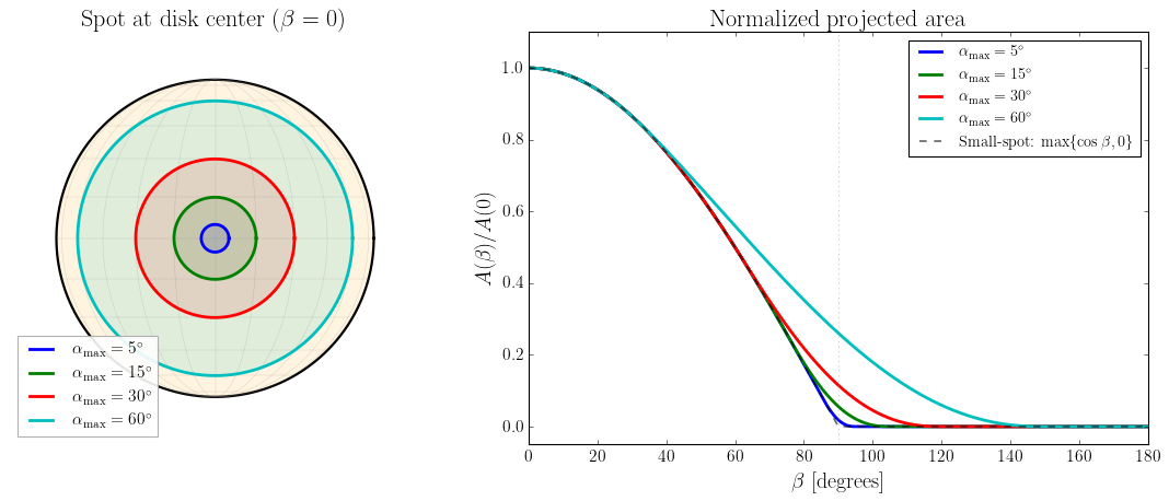
3. Visualize the projected area#
First, we show the size of spots with different angular radii \(\alpha_{\max}\) on the stellar disk at \(\beta = 0\) (disk center). Then we compare the exact projected area to the small-spot approximation as a function of \(\beta\).
# Spot sizes on the stellar disk at beta=0 (disk center)
alphas_deg = [5, 15, 30, 60]
colors_disk = ['C0', 'C1', 'C2', 'C3']

fig, (ax_disk, ax_area) = plt.subplots(1, 2, figsize=(14, 6),
                                        gridspec_kw={'width_ratios': [1, 1.3]})

# -- Left: stellar disk with spots at disk center --
th = np.linspace(0, 2 * np.pi, 500)
ax_disk.plot(np.cos(th), np.sin(th), 'k-', lw=2)
ax_disk.fill(np.cos(th), np.sin(th), color='#FFF4E0', zorder=0)

# Latitude/longitude grid
for lat_deg in np.arange(-75, 90, 15):
    lat = np.radians(lat_deg)
    lon = np.linspace(-np.pi / 2, np.pi / 2, 500)
    y_proj = np.cos(lat) * np.sin(lon)
    z_proj = np.sin(lat)
    ax_disk.plot(y_proj, np.full_like(y_proj, z_proj),
                 color='gray', lw=0.3, alpha=0.4)
for lon_deg in np.arange(-75, 90, 15):
    lon = np.radians(lon_deg)
    lat = np.linspace(-np.pi / 2, np.pi / 2, 500)
    y_proj = np.cos(lat) * np.sin(lon)
    z_proj = np.sin(lat)
    ax_disk.plot(y_proj, z_proj, color='gray', lw=0.3, alpha=0.4)

# Draw spot circles at disk center
for alpha_deg, color in zip(alphas_deg, colors_disk):
    alpha = np.radians(alpha_deg)
    r_spot = np.sin(alpha)  # projected radius on the unit disk
    spot_th = np.linspace(0, 2 * np.pi, 300)
    ax_disk.plot(r_spot * np.cos(spot_th), r_spot * np.sin(spot_th),
                 color=color, lw=2.5,
                 label=rf'$\alpha_{{\max}} = {alpha_deg}^\circ$', zorder=3)
    ax_disk.fill(r_spot * np.cos(spot_th), r_spot * np.sin(spot_th),
                 color=color, alpha=0.12, zorder=2)

ax_disk.set_xlim(-1.3, 1.3)
ax_disk.set_ylim(-1.3, 1.3)
ax_disk.set_aspect('equal')
ax_disk.set_title(r'Spot at disk center ($\beta = 0$)')
ax_disk.legend(loc='lower left', framealpha=0.9, edgecolor='#AAAAAA')
ax_disk.axis('off')

# -- Right: normalized projected area A(beta)/A(0) vs beta --
beta = np.linspace(0, np.pi, 500)
for alpha_deg, color in zip(alphas_deg, colors_disk):
    alpha = np.radians(alpha_deg)
    A_exact = np.array(FullGeometryVisibilityFunction.projected_area(alpha, jnp.array(beta)))
    A_max = np.pi * np.sin(alpha)**2
    ax_area.plot(np.degrees(beta), A_exact / A_max,
                 color=color, lw=2.5,
                 label=rf'$\alpha_{{\max}} = {alpha_deg}^\circ$')

# Small-spot approximation
ax_area.plot(np.degrees(beta), np.maximum(np.cos(beta), 0),
             'k--', lw=1.5, alpha=0.6,
             label=r'Small-spot: $\max\{\cos\beta, 0\}$')

ax_area.axvline(90, color='gray', ls=':', lw=0.8, alpha=0.5)
ax_area.set_xlabel(r'$\beta$ [degrees]')
ax_area.set_ylabel(r'$A(\beta) / A(0)$')
ax_area.set_title('Normalized projected area')
ax_area.legend(fontsize=13, loc='upper right')
ax_area.set_xlim(0, 180)
ax_area.set_ylim(-0.05, 1.1)

plt.tight_layout()
plt.show()
beta = jnp.linspace(0, jnp.pi, 500)
alphas = [0.05, 0.1, 0.3, 0.6, 1.0]  # radians

fig, axes = plt.subplots(1, 2, figsize=(14, 5))

for alpha in alphas:
    A_exact = np.array(FullGeometryVisibilityFunction.projected_area(alpha, beta))
    A_approx = np.pi * np.sin(alpha)**2 * np.clip(np.cos(beta), 0, None)

    label = rf"$\alpha = {np.degrees(alpha):.0f}^\circ$ ({alpha:.2f} rad)"
    axes[0].plot(np.degrees(np.array(beta)), A_exact, label=label)
    axes[0].plot(np.degrees(np.array(beta)), A_approx, "--", color="gray", alpha=0.4)

    # Relative error (avoid division by zero)
    mask = A_exact > 1e-10
    rel_err = np.full_like(A_exact, np.nan)
    rel_err[mask] = np.abs(A_exact[mask] - A_approx[mask]) / A_exact[mask]
    axes[1].plot(np.degrees(np.array(beta)), rel_err * 100, label=label)

axes[0].set_xlabel(r"$\beta$ [degrees]")
axes[0].set_ylabel(r"Projected area $A$")
axes[0].set_title("Solid: exact, Dashed: small-spot approx")
axes[0].legend()

axes[1].set_xlabel(r"$\beta$ [degrees]")
axes[1].set_ylabel(r"Relative error [\%]")
axes[1].set_title("Approximation error")
axes[1].set_ylim(0, 100)
axes[1].legend()

plt.tight_layout()
plt.show()
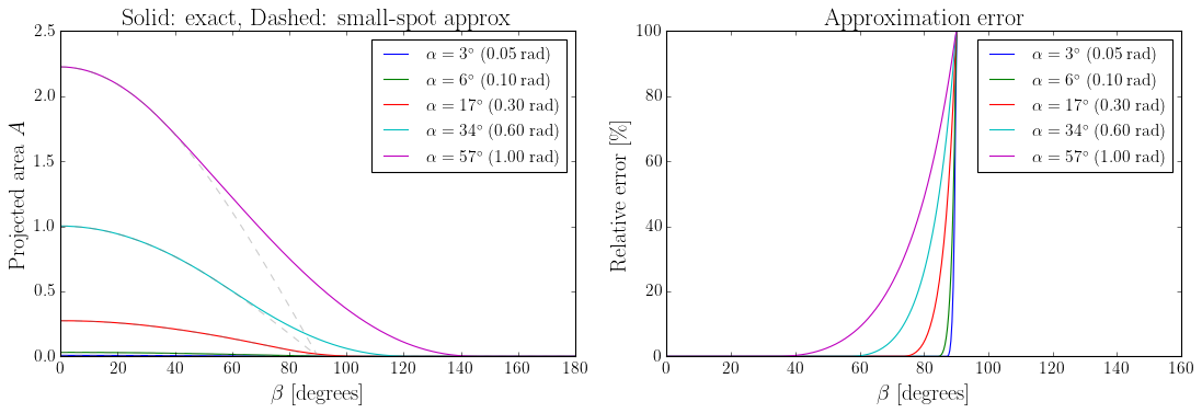
The small-spot approximation is accurate for the fully visible region but completely misses the partial-visibility transition near the limb (\(\beta \approx 90°\)). For small spots (\(\alpha \lesssim 6°\)), the partial-visibility window is so narrow that this error is negligible; for large spots, the smooth transition matters.
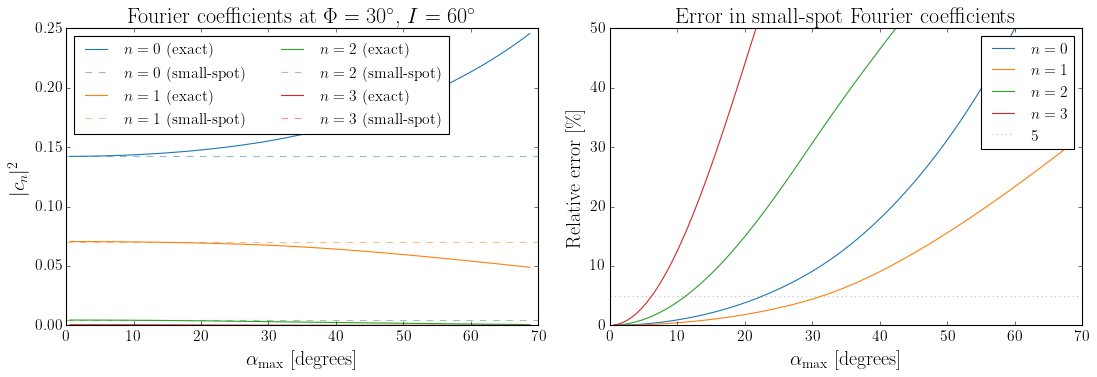
4. Compare Fourier coefficients \(|c_n|^2\)#
The analytic kernel depends on the squared Fourier coefficients \(|c_n|^2\). Compare the closed-form (small-spot) coefficients to the numerically computed (exact geometry) coefficients as a function of spot size.
inc = np.pi / 3
phi = np.pi / 6  # 30 deg latitude
n_harmonics = 3

alpha_grid = np.linspace(0.01, 1.2, 100)  # 0.6 deg to 69 deg

cn_small_spot = np.array([
    VisibilityFunction(peq=10.0, kappa=0.0, inc=inc).cn_squared(phi, n_harmonics)
    for _ in alpha_grid
])  # shape (n_alpha, n_harmonics+1) — independent of alpha

cn_exact = np.array([
    FullGeometryVisibilityFunction(
        peq=10.0, kappa=0.0, inc=inc, alpha_ref=a
    ).cn_squared(phi, n_harmonics)
    for a in alpha_grid
])  # shape (n_alpha, n_harmonics+1)

fig, axes = plt.subplots(1, 2, figsize=(14, 5))
colors = plt.cm.tab10.colors

for n in range(n_harmonics + 1):
    axes[0].plot(np.degrees(alpha_grid), cn_exact[:, n],
                 color=colors[n], label=f"$n={n}$ (exact)")
    axes[0].axhline(cn_small_spot[0, n], color=colors[n], ls="--", alpha=0.5,
                    label=f"$n={n}$ (small-spot)")

axes[0].set_xlabel(r"$\alpha_{\max}$ [degrees]")
axes[0].set_ylabel(r"$|c_n|^2$")
axes[0].set_title(rf"Fourier coefficients at $\Phi = {np.degrees(phi):.0f}^\circ$, $I = {np.degrees(inc):.0f}^\circ$")
axes[0].legend(fontsize=14, ncol=2, loc="upper left")

# Relative error in each coefficient
for n in range(n_harmonics + 1):
    ref = cn_small_spot[0, n]
    if ref > 1e-15:
        rel_err = np.abs(cn_exact[:, n] - ref) / ref * 100
        axes[1].plot(np.degrees(alpha_grid), rel_err,
                     color=colors[n], label=f"$n={n}$")

axes[1].axhline(5, color="gray", ls=":", alpha=0.5, label="5% threshold")
axes[1].set_xlabel(r"$\alpha_{\max}$ [degrees]")
axes[1].set_ylabel(r"Relative error [\%]")
axes[1].set_title("Error in small-spot Fourier coefficients")
axes[1].legend()
axes[1].set_ylim(0, 50)

plt.tight_layout()
plt.show()
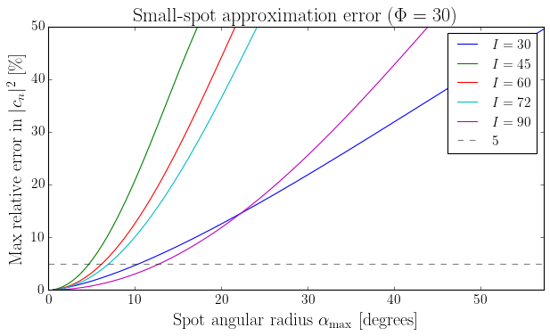
5. Divergence threshold: where does the approximation break down?#
Find the spot size \(\alpha_{\max}\) at which the small-spot Fourier coefficients deviate from the exact values by more than 5%, as a function of inclination.
alpha_fine = np.linspace(0.01, 1.0, 200)
inclinations = np.array([np.pi / 6, np.pi / 4, np.pi / 3, np.pi / 2.5, np.pi / 2])
phi_test = np.pi / 6
threshold = 0.05  # 5%

fig, ax = plt.subplots(figsize=(8, 5))

for inc in inclinations:
    cn_ref = np.array(
        VisibilityFunction(peq=10.0, kappa=0.0, inc=inc).cn_squared(phi_test, 3)
    )

    cn_ex = np.array([
        FullGeometryVisibilityFunction(
            peq=10.0, kappa=0.0, inc=inc, alpha_ref=a
        ).cn_squared(phi_test, 3)
        for a in alpha_fine
    ])

    # Max relative error across all harmonics with nonzero reference
    nonzero = cn_ref > 1e-15
    max_rel_err = np.max(
        np.abs(cn_ex[:, nonzero] - cn_ref[nonzero]) / cn_ref[nonzero],
        axis=1,
    )

    ax.plot(np.degrees(alpha_fine), max_rel_err * 100,
            label=rf"$I = {np.degrees(inc):.0f}°$")

ax.axhline(threshold * 100, color="k", ls="--", alpha=0.5, label=f"{threshold*100:.0f}% threshold")
ax.set_xlabel(r"Spot angular radius $\alpha_{\max}$ [degrees]")
ax.set_ylabel("Max relative error in $|c_n|^2$ [\%]")
ax.set_title(rf"Small-spot approximation error ($\Phi = {np.degrees(phi_test):.0f}°$)")
ax.legend()
ax.set_ylim(0, 50)
ax.set_xlim(0, np.degrees(alpha_fine[-1]))
plt.tight_layout()
plt.show()
<>:32: SyntaxWarning: "\%" is an invalid escape sequence. Such sequences will not work in the future. Did you mean "\\%"? A raw string is also an option.
<>:32: SyntaxWarning: "\%" is an invalid escape sequence. Such sequences will not work in the future. Did you mean "\\%"? A raw string is also an option.
/tmp/ipykernel_2695030/726072386.py:32: SyntaxWarning: "\%" is an invalid escape sequence. Such sequences will not work in the future. Did you mean "\\%"? A raw string is also an option.
  ax.set_ylabel("Max relative error in $|c_n|^2$ [\%]")
print(f"{'Inclination':>14s}  {'alpha_max (5% threshold)':>26s}")
print("-" * 44)

for inc in inclinations:
    cn_ref = np.array(
        VisibilityFunction(peq=10.0, kappa=0.0, inc=inc).cn_squared(phi_test, 3)
    )
    cn_ex = np.array([
        FullGeometryVisibilityFunction(
            peq=10.0, kappa=0.0, inc=inc, alpha_ref=a
        ).cn_squared(phi_test, 3)
        for a in alpha_fine
    ])

    nonzero = cn_ref > 1e-15
    max_rel_err = np.max(
        np.abs(cn_ex[:, nonzero] - cn_ref[nonzero]) / cn_ref[nonzero],
        axis=1,
    )

    idx = np.argmax(max_rel_err > threshold)
    if max_rel_err[idx] > threshold:
        alpha_thresh = np.degrees(alpha_fine[idx])
        print(f"{np.degrees(inc):>12.0f}°  {alpha_thresh:>22.1f}°")
    else:
        print(f"{np.degrees(inc):>12.0f}°  {'> 57°':>22s}")
   Inclination    alpha_max (5% threshold)
--------------------------------------------
          30°                    10.5°
          45°                     4.8°
          60°                     6.3°
          72°                     7.1°
          90°                    13.1°
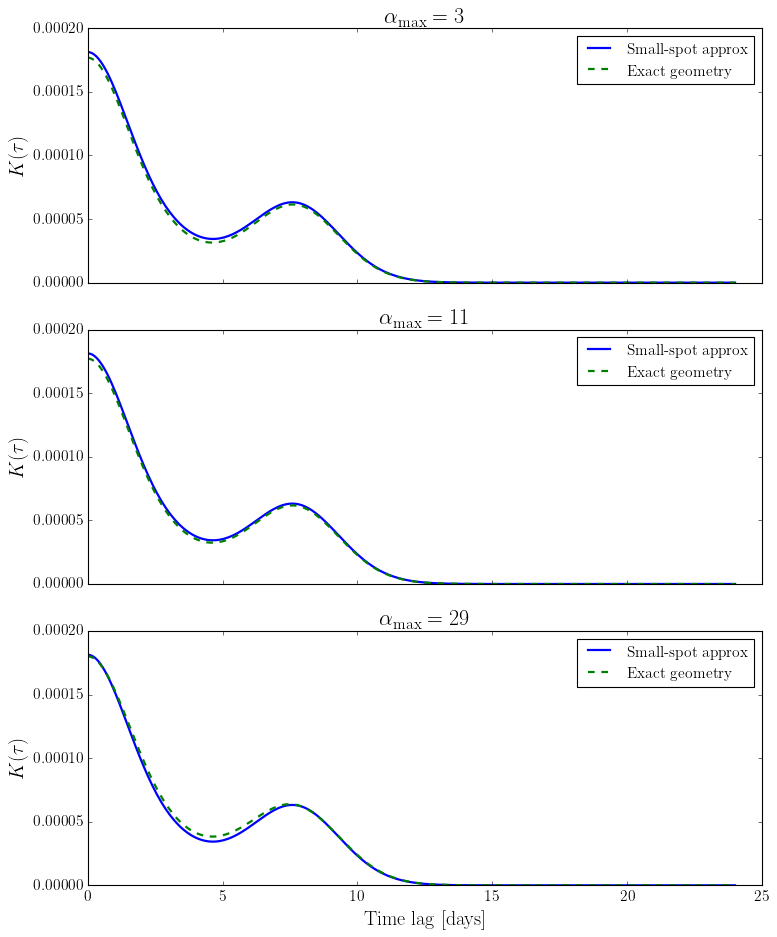
6. Compare GP kernels#
Build an AnalyticKernel with each visibility function and compare the resulting covariance kernels.
env = TrapezoidSymmetricEnvelope(lspot=10.0, tau_spot=3.0)
peq, kappa, inc = 8.0, 0.2, np.pi / 3

alphas_compare = [0.05, 0.2, 0.5]
lag = np.linspace(0, 3 * peq, 300)

fig, axes = plt.subplots(len(alphas_compare), 1, figsize=(10, 4 * len(alphas_compare)),
                         sharex=True)

for ax, alpha in zip(axes, alphas_compare):
    # Small-spot kernel
    vis_small = VisibilityFunction(peq=peq, kappa=kappa, inc=inc)
    model_small = SpotEvolutionModel(envelope=env, visibility=vis_small, sigma_k=0.01)
    K_small = AnalyticKernel(model_small).kernel(lag)

    # Full geometry kernel
    vis_full = FullGeometryVisibilityFunction(
        peq=peq, kappa=kappa, inc=inc, alpha_ref=alpha)
    model_full = SpotEvolutionModel(envelope=env, visibility=vis_full, sigma_k=0.01)
    K_full = AnalyticKernel(model_full).kernel(lag)

    ax.plot(lag, np.array(K_small), label="Small-spot approx", lw=2)
    ax.plot(lag, np.array(K_full), "--", label="Exact geometry", lw=2)
    ax.set_ylabel(r"$K(\tau)$")
    ax.set_title(rf"$\alpha_{{\max}} = {np.degrees(alpha):.0f}°$")
    ax.legend()

axes[-1].set_xlabel("Time lag [days]")
plt.tight_layout()
plt.show()
7. Computation speed comparison#
The small-spot approximation uses closed-form Fourier coefficients \(c_n(I, \Phi)\), while the full geometry computes them numerically via DFT at each latitude. How much does this cost in practice?
We benchmark three operations:
cn_squared— computing the Fourier coefficients at a single latitudeAnalyticKernel.kernel()— full kernel evaluation (latitude-averaged) on a lag arrayGPSolver.log_posterior()— full log-likelihood evaluation (kernel + Cholesky + solve)
import time
import jax
from spotgp import GPSolver

jax.config.update("jax_enable_x64", True)

env = TrapezoidSymmetricEnvelope(lspot=10.0, tau_spot=3.0)
peq, kappa, inc = 8.0, 0.0, np.pi / 3
n_harmonics = 3
phi_test = np.pi / 6

vis_small = VisibilityFunction(peq=peq, kappa=kappa, inc=inc)
vis_full = FullGeometryVisibilityFunction(peq=peq, kappa=kappa, inc=inc, alpha_ref=0.1)

# --- 1. cn_squared benchmark ---
n_repeat = 200

# Warmup
_ = vis_small.cn_squared(phi_test, n_harmonics)
_ = vis_full.cn_squared(phi_test, n_harmonics)

t0 = time.perf_counter()
for _ in range(n_repeat):
    _ = vis_small.cn_squared(phi_test, n_harmonics)
t_cn_small = (time.perf_counter() - t0) / n_repeat

t0 = time.perf_counter()
for _ in range(n_repeat):
    _ = vis_full.cn_squared(phi_test, n_harmonics)
t_cn_full = (time.perf_counter() - t0) / n_repeat

print("=== cn_squared (single latitude) ===")
print(f"  Small-spot:     {t_cn_small*1e3:.3f} ms")
print(f"  Full geometry:  {t_cn_full*1e3:.3f} ms")
print(f"  Slowdown:       {t_cn_full/t_cn_small:.1f}x")

# --- 2. AnalyticKernel.kernel() benchmark ---
lag = np.linspace(0, 3 * peq, 500)

model_small = SpotEvolutionModel(envelope=env, visibility=vis_small, sigma_k=0.01)
model_full = SpotEvolutionModel(envelope=env, visibility=vis_full, sigma_k=0.01)

ak_small = AnalyticKernel(model_small, n_harmonics=n_harmonics)
ak_full = AnalyticKernel(model_full, n_harmonics=n_harmonics)

# Warmup
_ = ak_small.kernel(lag)
_ = ak_full.kernel(lag)

n_repeat_k = 20

t0 = time.perf_counter()
for _ in range(n_repeat_k):
    _ = ak_small.kernel(lag)
t_k_small = (time.perf_counter() - t0) / n_repeat_k

t0 = time.perf_counter()
for _ in range(n_repeat_k):
    _ = ak_full.kernel(lag)
t_k_full = (time.perf_counter() - t0) / n_repeat_k

print(f"\n=== AnalyticKernel.kernel() ({len(lag)} lags) ===")
print(f"  Small-spot:     {t_k_small*1e3:.1f} ms")
print(f"  Full geometry:  {t_k_full*1e3:.1f} ms")
print(f"  Slowdown:       {t_k_full/t_k_small:.1f}x")

# --- 3. GPSolver.log_posterior() benchmark ---
tsim_values = [100, 500, 1000]
tsamp = 0.5
sigma_n = 1e-3
n_repeat_gp = 5

print(f"\n=== GPSolver.log_posterior() (banded Cholesky) ===")
print(f"{'N':>8s}  {'Small-spot':>12s}  {'Full geom.':>12s}  {'Slowdown':>10s}")
print("-" * 48)

for tsim in tsim_values:
    x_obs = np.arange(0, tsim, tsamp)
    N = len(x_obs)
    y_obs = np.zeros(N)
    yerr_obs = np.full(N, sigma_n)

    hparam = dict(peq=peq, kappa=kappa, inc=inc, lspot=10.0, tau=3.0, sigma_k=0.01)

    # Small-spot solver
    gp_s = GPSolver(x_obs, y_obs, yerr_obs, model_small,
                    matrix_solver="cholesky_banded", fit_sigma_n=False,
                    n_harmonics=n_harmonics)
    theta_s = gp_s.theta0
    # Warmup
    for _ in range(2):
        _ = gp_s.log_posterior(theta_s).block_until_ready()
    t0 = time.perf_counter()
    for _ in range(n_repeat_gp):
        _ = gp_s.log_posterior(theta_s).block_until_ready()
    t_gp_small = (time.perf_counter() - t0) / n_repeat_gp

    # Full geometry solver
    gp_f = GPSolver(x_obs, y_obs, yerr_obs, model_full,
                    matrix_solver="cholesky_banded", fit_sigma_n=False,
                    n_harmonics=n_harmonics)
    theta_f = gp_f.theta0
    for _ in range(2):
        _ = gp_f.log_posterior(theta_f).block_until_ready()
    t0 = time.perf_counter()
    for _ in range(n_repeat_gp):
        _ = gp_f.log_posterior(theta_f).block_until_ready()
    t_gp_full = (time.perf_counter() - t0) / n_repeat_gp

    print(f"{N:>8d}  {t_gp_small*1e3:>10.1f} ms  {t_gp_full*1e3:>10.1f} ms  {t_gp_full/t_gp_small:>8.1f}x")
=== cn_squared (single latitude) ===
  Small-spot:     0.339 ms
  Full geometry:  1.041 ms
  Slowdown:       3.1x

=== AnalyticKernel.kernel() (500 lags) ===
  Small-spot:     89.0 ms
  Full geometry:  80.9 ms
  Slowdown:       0.9x

=== GPSolver.log_posterior() (banded Cholesky) ===
       N    Small-spot    Full geom.    Slowdown
------------------------------------------------
Banded Cholesky: bandwidth=80, N=200, sparsity=59.5%
Banded Cholesky: bandwidth=80, N=200, sparsity=59.5%
     200         6.4 ms         6.9 ms       1.1x
Banded Cholesky: bandwidth=80, N=1000, sparsity=91.9%
Banded Cholesky: bandwidth=80, N=1000, sparsity=91.9%
    1000        37.7 ms        36.7 ms       1.0x
Banded Cholesky: bandwidth=80, N=2000, sparsity=96.0%
Banded Cholesky: bandwidth=80, N=2000, sparsity=96.0%
    2000        90.0 ms        95.1 ms       1.1x
The cn_squared computation is significantly slower for the full geometry model because it evaluates the exact piecewise area function on a longitude grid and computes a DFT, whereas the small-spot approximation uses closed-form expressions. However, at the GPSolver level the difference is smaller because the Cholesky factorization dominates the total cost for large \(N\). The kernel evaluation overhead from the full geometry becomes a smaller fraction of the total wall-clock time as the dataset grows.
Summary#
The small-spot approximation (\(A \approx \pi\alpha^2 \cos\beta\)) is accurate for spot radii \(\alpha_{\max} \lesssim 10\text{--}15°\), which covers the vast majority of observed starspots.
For larger spots, the partial-visibility window near the stellar limb becomes significant, and the exact piecewise geometry should be used.
To implement a custom visibility function, subclass
VisibilityFunctionand overridecn_squared(). If the Fourier coefficients don’t have a closed form, compute them numerically via DFT as shown above.The
FullGeometryVisibilityFunctionis available inspotgpas a built-in alternative to the base class.