Data Preprocessing

The TimeSeriesData class provides a standard container for photometric time series with built-in preprocessing, PSD, and ACF computation.

Sections

1. Creating a TimeSeriesData from simulated data

2. Loading Kepler data via lightkurve

3. Normalization, sigma clipping, PSD, and ACF

import sys
sys.path.append("../..")

import numpy as np
import matplotlib.pyplot as plt

plt.rcParams.update({                                                                                  
    "font.size":        16,   # base font size                                                         
    "axes.titlesize":   20,   # axes title                                                             
    "axes.labelsize":   18,   # x/y axis labels                                                        
    "xtick.labelsize":  14,   # x tick labels                                                          
    "ytick.labelsize":  14,   # y tick labels                                                          
    "legend.fontsize":  14,                                                                            
    "figure.titlesize": 22,   # suptitle
    "axes.formatter.useoffset": False,  # disable scientific notation offset                                                   
})  

from spotgp import TimeSeriesData

---

1. Simulated data

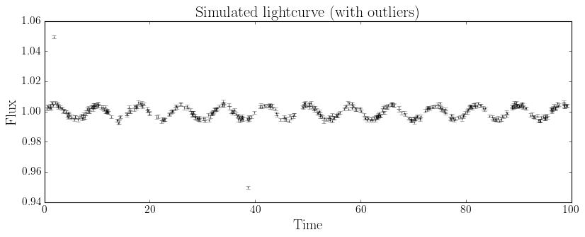
Create a synthetic lightcurve with a periodic signal, noise, and a few outliers.

np.random.seed(42)

N = 500
t = np.sort(np.random.uniform(0, 100, N))  # irregular sampling
period = 8.0
flux = 1.0 + 0.005 * np.sin(2 * np.pi * t / period) + 0.001 * np.random.randn(N)
flux_err = np.full(N, 0.001)

# Inject some outliers and NaNs
flux[10] = 1.05
flux[200] = 0.95
flux[300] = np.nan

ts = TimeSeriesData(t, flux, flux_err)
print(ts)
print(f"Median flux: {np.median(ts.y):.6f}")

TimeSeriesData(N=499, baseline=98.79, median_dt=0.1299)
Median flux: 1.000000

The constructor automatically:

• Removed the NaN entry (N went from 500 to 499)

• Normalized the flux so the median is 1.0

Plot the raw time series

ts.plot()
plt.title("Simulated lightcurve (with outliers)")
plt.show()

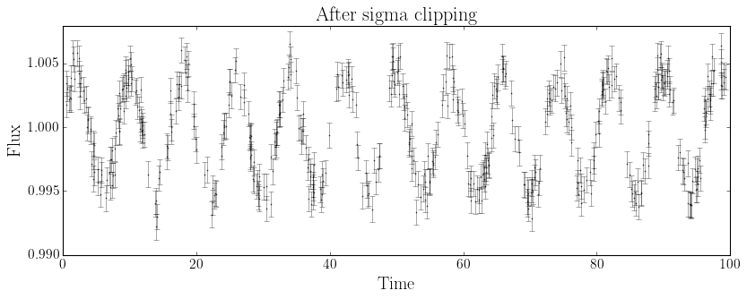
Sigma clipping

Remove the outliers with sigma_clip():

print(f"Before clipping: N = {ts.N}")
ts.sigma_clip(lower=3, upper=3)
print(f"After clipping:  N = {ts.N}")

ts.plot()
plt.title("After sigma clipping")
plt.show()

Before clipping: N = 499
After clipping:  N = 497

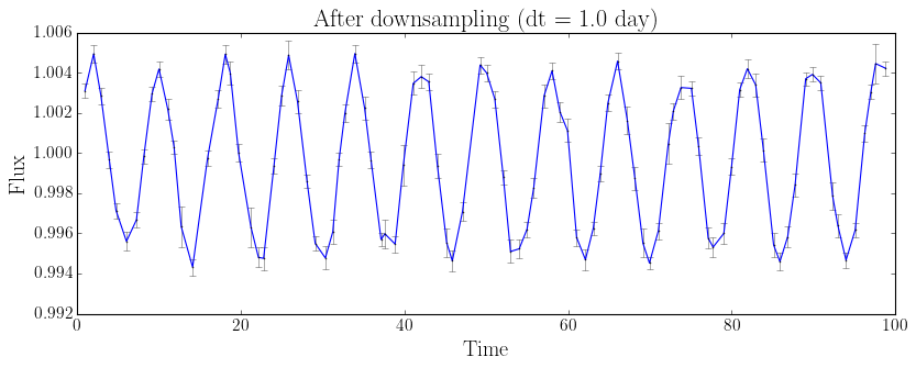
Downsampling

Bin the time series into uniform time bins using inverse-variance weighted averaging. This reduces the number of points while preserving the signal and correctly propagating uncertainties.

print(f"Before downsampling: N = {ts.N}, median dt = {ts.median_dt:.4f}")
ts.downsample(dt=1.0)
print(f"After downsampling:  N = {ts.N}, median dt = {ts.median_dt:.4f}")

ts.plot()
plt.plot(ts.x, ts.y)
plt.title("After downsampling (dt = 1.0 day)")
plt.show()

Before downsampling: N = 497, median dt = 0.1311
After downsampling:  N = 97, median dt = 0.9924

PSD and ACF

Compute and plot the power spectral density and autocorrelation function:

fig, axes = plt.subplots(1, 2, figsize=(14, 4))

ts.plot_psd(ax=axes[0])
axes[0].axvline(1.0 / period, color="r", ls="--", label=f"Injected: $f = 1/{period:.0f}$ d$^{{-1}}$")
axes[0].legend()
axes[0].set_title("Lomb-Scargle PSD")

ts.plot_acf(ax=axes[1], n_bins=100, max_lag=40)
for i in range(1, 5):
    axes[1].axvline(i * period, color="r", ls="--", alpha=0.4)
axes[1].set_title("Autocorrelation function")

plt.tight_layout()
plt.show()

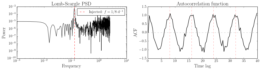
The PSD peaks at the injected frequency (\(1/8\) d\(^{-1}\)) and the ACF shows periodicity at multiples of 8 days.

---

2. Kepler data with lightkurve

Load a Kepler quarter for a known active star and preprocess it with TimeSeriesData.

Note

This section requires lightkurve. Install it with pip install lightkurve.

import lightkurve as lk

# Download a single Kepler quarter for a spotted star
search = lk.search_lightcurve("KIC 7985370", mission="Kepler", cadence="long", quarter=5)
lc = search.download()
lc.head()

KeplerLightCurve length=5 LABEL="KIC 7985370" QUARTER=5 AUTHOR=Kepler FLUX_ORIGIN=pdcsap_flux

time	flux	flux_err	quality	timecorr	centroid_col	centroid_row	cadenceno	sap_flux	sap_flux_err	sap_bkg	sap_bkg_err	pdcsap_flux	pdcsap_flux_err	sap_quality	psf_centr1	psf_centr1_err	psf_centr2	psf_centr2_err	mom_centr1	mom_centr1_err	mom_centr2	mom_centr2_err	pos_corr1	pos_corr2
	electron / s	electron / s		d	pix	pix		electron / s	electron / s	electron / s	electron / s	electron / s	electron / s		pix	pix	pix	pix	pix	pix	pix	pix	pix	pix
Time	float32	float32	int32	float32	float64	float64	int32	float32	float32	float32	float32	float32	float32	int32	float64	float32	float64	float32	float64	float32	float64	float32	float32	float32
443.48970645623194	———	———	10000	-1.448464e-03	319.40248	398.02002	16373	1.5593305e+06	3.1996595e+01	8.0061802e+03	1.6346836e+00	———	———	10000	———	———	———	———	319.40248	2.0221185e-05	398.02002	2.9403081e-05	-4.5754738e-02	4.8700325e-02
443.51014069512166	1.5641606e+06	3.2047684e+01	10000000010000	-1.447925e-03	319.40256	398.02001	16374	1.5606115e+06	3.2009605e+01	8.0055918e+03	1.6347697e+00	1.5641606e+06	3.2047684e+01	10000000010000	———	———	———	———	319.40256	2.0208812e-05	398.02001	2.9394563e-05	-4.5619853e-02	4.9024601e-02
443.5305747343591	1.5655112e+06	3.2063877e+01	10000000010000	-1.447386e-03	319.40289	398.01947	16375	1.5619460e+06	3.2023129e+01	8.0033838e+03	1.6351467e+00	1.5655112e+06	3.2063877e+01	10000000010000	———	———	———	———	319.40289	2.0198473e-05	398.01947	2.9383289e-05	-4.5340929e-02	4.8469041e-02
443.55100887370645	1.5667932e+06	3.2078529e+01	10000	-1.446846e-03	319.40306	398.01928	16376	1.5632136e+06	3.2036301e+01	8.0128496e+03	1.6329130e+00	1.5667932e+06	3.2078529e+01	10000	———	———	———	———	319.40306	2.0186624e-05	398.01928	2.9375227e-05	-4.5147281e-02	4.8476472e-02
443.5714431134111	1.5680732e+06	3.2089455e+01	10010000	-1.446307e-03	319.40302	398.01933	16377	1.5645386e+06	3.2048767e+01	8.0063745e+03	1.6347470e+00	1.5680732e+06	3.2089455e+01	10010000	———	———	———	———	319.40302	2.0174755e-05	398.01933	2.9367231e-05	-4.5176014e-02	4.8612297e-02

ts_kepler = TimeSeriesData.from_lightkurve(lc, normalize=True)
print(ts_kepler)

TimeSeriesData(N=4486, baseline=94.65, median_dt=0.0204)

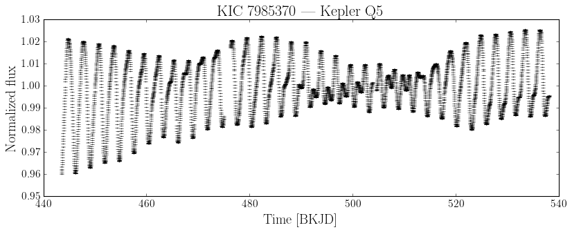
Plot the raw lightcurve

ts_kepler.plot(xlabel="Time [BKJD]", ylabel="Normalized flux")
plt.title("KIC 7985370 — Kepler Q5")
plt.show()

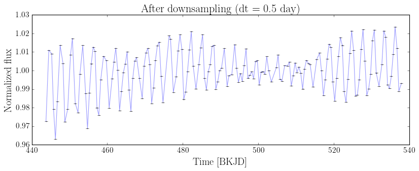
Downsample

Kepler long-cadence data has ~30 min sampling. Downsample to 1-day bins to speed up GP fitting:

print(f"Before downsampling: N = {ts_kepler.N}, median dt = {ts_kepler.median_dt:.4f}")
ts_kepler.downsample(dt=0.5)
print(f"After downsampling:  N = {ts_kepler.N}, median dt = {ts_kepler.median_dt:.4f}")

ts_kepler.plot(xlabel="Time [BKJD]", ylabel="Normalized flux")
plt.plot(ts_kepler.x, ts_kepler.y, alpha=0.4)
plt.title("After downsampling (dt = 0.5 day)")
plt.show()

Before downsampling: N = 187, median dt = 0.5006
After downsampling:  N = 169, median dt = 0.5006

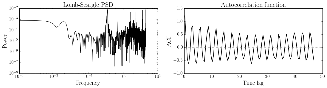
PSD and ACF

fig, axes = plt.subplots(1, 2, figsize=(14, 4))

ts_kepler.plot_psd(ax=axes[0])
axes[0].set_title("Lomb-Scargle PSD")

ts_kepler.plot_acf(ax=axes[1], n_bins=100)
axes[1].set_title("Autocorrelation function")

plt.tight_layout()
plt.show()

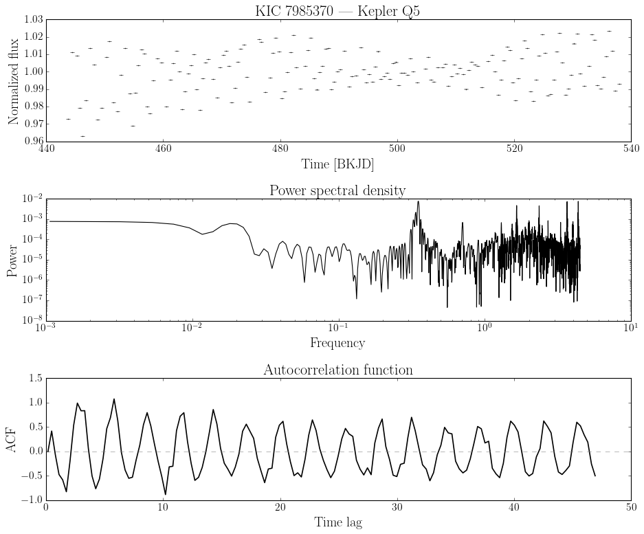
Summary panel

A combined three-panel view of the data:

fig, axes = plt.subplots(3, 1, figsize=(12, 10))

ts_kepler.plot(ax=axes[0], xlabel="Time [BKJD]", ylabel="Normalized flux")
axes[0].set_title("KIC 7985370 — Kepler Q5")

ts_kepler.plot_psd(ax=axes[1])
axes[1].set_title("Power spectral density")

ts_kepler.plot_acf(ax=axes[2], n_bins=150)
axes[2].set_title("Autocorrelation function")

plt.tight_layout()
plt.show()

---

API summary

Method	Description
TimeSeriesData(x, y, yerr)	Create from arrays (auto-removes NaN, normalizes by default)
TimeSeriesData.from_lightkurve(lc)	Create from a lightkurve.LightCurve
.normalize()	Divide flux by median
.sigma_clip(lower, upper)	Remove outliers beyond N-sigma
.downsample(dt)	Bin into non-overlapping intervals with inverse-variance weighted mean
.compute_psd()	Lomb-Scargle PSD
.compute_acf()	Binned empirical ACF
.plot()	Plot time series with error bars
.plot_psd()	Plot PSD (log-log by default)
.plot_acf()	Plot ACF