Time Domain

In this tutorial we explore how the two core physical components of the SpotEvolutionModel work independently, and then how they combine to produce a realistic stellar lightcurve.

SpotEvolutionModel

The SpotEvolutionModel decomposes starspot-driven photometric variability into two separable components:

• Envelope \(\Gamma(t)\): describes how an individual spot grows and decays over time — the birth/death cycle of a spot.

• Visibility \(\Pi(t)\): describes how the projected flux contribution of a spot changes as the star rotates — the rotational modulation.

The full statistical GP kernel is a product of both effects. Here we isolate each one to build intuition before combining them.

import sys
import numpy as np
import matplotlib.pyplot as plt
from IPython.display import HTML

sys.path.append("../..")
from spotgp import (
    TrapezoidSymmetricEnvelope,
    VisibilityFunction,
    SpotEvolutionModel,
    LightcurveModel,
)

np.random.seed(42)

1. Envelope Model \(\Gamma(t)\): spot growth and decay

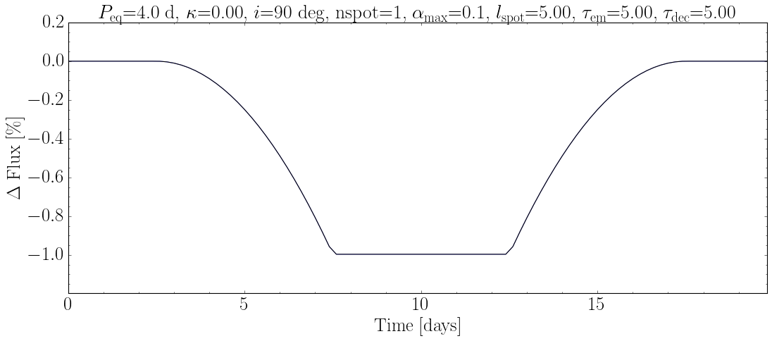
The envelope function \(\Gamma(t)\) describes the normalized spot area as a function of time relative to the spot’s peak size. It captures the growth and decay lifecycle of a single spot: a linear rise to maximum area, a plateau, and a linear decay back to zero.

Here we use the symmetric trapezoid envelope, parameterized by:

• lspot \(= \ell\) — plateau duration (days the spot spends at peak size)

• tau_spot \(= \tau\) — rise/decay timescale (days to grow from zero to peak, and peak back to zero)

Setting visibility=None isolates the envelope: the star does not rotate, and the spot sits fixed at disk center. Only the changing spot size modulates the flux.

envelope = TrapezoidSymmetricEnvelope(
    lspot=5.0,      # plateau duration [days]
    tau_spot=5.0,    # rise/decay timescale [days]
)

envelope_only_model = SpotEvolutionModel(
    envelope=envelope,
    visibility=None,
    sigma_k=0.1
)

The analytic expressions for \(\Gamma(t)\), its Fourier transform \(\hat{\Gamma}(\omega)\), and the autocorrelation \(R_\Gamma(\tau)\) are:

env_equations = envelope_only_model.get_sympy()

\[\displaystyle \textbf{TrapezoidSymmetricEnvelope} \text{[user defined]}\]

\[\begin{split}\displaystyle \Gamma(t) = \begin{cases} 0 & \text{for}\: t < - \frac{\ell}{2} - \tau_{\rm spot} \\\frac{\left(\frac{\ell}{2} + \tau_{\rm spot} + t\right)^{2}}{\tau_{\rm spot}^{2}} & \text{for}\: t < - \frac{\ell}{2} \\1 & \text{for}\: t \leq \frac{\ell}{2} \\\frac{\left(\frac{\ell}{2} + \tau_{\rm spot} - t\right)^{2}}{\tau_{\rm spot}^{2}} & \text{for}\: t < \frac{\ell}{2} + \tau_{\rm spot} \\0 & \text{otherwise} \end{cases}\end{split}\]

\[\displaystyle \hat{\Gamma}(\omega) = \frac{4 \left(\omega \tau_{\rm spot} \cos{\left(\frac{\ell \omega}{2} \right)} + \sin{\left(\frac{\ell \omega}{2} \right)} - \sin{\left(\frac{\ell \omega}{2} + \omega \tau_{\rm spot} \right)}\right)}{\omega^{3} \tau_{\rm spot}^{2}}\]

\[\displaystyle R_{\Gamma}(\tau) = \int\limits_{0}^{\infty} \Gamma{\left(t \right)} \Gamma{\left(\tau + t \right)}\, dt \quad \text{[numerical]}\]

\[\displaystyle \textbf{VisibilityFunction} \text{ [not specified]}\]

\[\displaystyle \textbf{LatitudeDistributionFunction} \text{[default]}\]

\[\displaystyle p(\phi) = 1\]

The simulated lightcurve below shows a single spot placed at disk center (long=0, lat=0) peaking at tmax=10 days. The flux dip follows the trapezoid shape of \(\Gamma(t)\) directly — rising, plateauing, then recovering.

lc_env = LightcurveModel.from_spot_model(
    spot_model=envelope_only_model,
    nspot=1,        # total number of spots to place
    tsim=20,       # simulation duration [days]
    tsamp=0.2,      # cadence [days]
    lat=0.0,
    long=0.0,
    tmax=10.0,
)

lc_env.plot_lightcurve()

anim_env = lc_env.animate_lightcurve(fps=20, duration=6)
HTML(anim_env.to_jshtml())

Once Loop Reflect

2. Visibility Function \(\Pi(t)\): rotational modulation

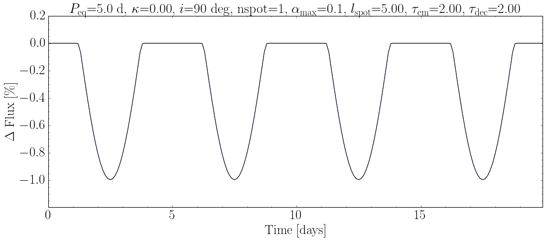
The visibility function encodes how the flux contribution of a spot varies as the star rotates. A spot on the near side of the star contributes more flux deficit than the same spot near the limb or hidden on the far side.

It is parameterized by:

• peq \(= P_\mathrm{eq}\) — equatorial rotation period [days]

• kappa \(= \kappa\) — differential rotation shear (0 = solid-body)

• inc \(= i\) — stellar inclination [rad] (\(i = \pi/2\) is edge-on)

Setting envelope=None isolates the visibility: the spot has a constant size at all times (alpha_max), and only the rotational modulation changes the flux. The spot is placed at long=0 (disk center at t=tmax) and lat=0 (equator).

visibility = VisibilityFunction(
    peq=5.0,         # equatorial rotation period [days]
    kappa=0.,        # differential rotation shear
    inc=np.pi / 2,   # stellar inclination [rad]
)

visibility_only_model = SpotEvolutionModel(
    envelope=None,
    visibility=visibility,
    sigma_k=0.1
)

vis_equations = visibility_only_model.get_sympy()

\[\displaystyle \textbf{EnvelopeFunction} \text{ [not specified]}\]

\[\displaystyle \textbf{VisibilityFunction} \text{[user defined]}\]

\[\displaystyle \omega_0(\phi) = \frac{2 \pi \left(- \kappa \sin^{2}{\left(\phi \right)} + 1\right)}{P_{\rm eq}}\]

\[\displaystyle a_0 = \sin{\left(\phi \right)} \cos{\left(i \right)}\]

\[\displaystyle a_1 = \sin{\left(i \right)} \cos{\left(\phi \right)}\]

\[\displaystyle \theta_v = \operatorname{acos}{\left(- \frac{a_{0}}{a_{1}} \right)}\]

\[\displaystyle c_0 = \frac{\theta_{v} a_{0} + a_{1} \sin{\left(\theta_{v} \right)}}{\pi}\]

\[\displaystyle c_1 = \frac{a_{0} \sin{\left(\theta_{v} \right)} + \frac{a_{1} \left(\theta_{v} + \sin{\left(\theta_{v} \right)} \cos{\left(\theta_{v} \right)}\right)}{2}}{\pi}\]

\[\displaystyle c_n \; (n \geq 2) = \frac{\frac{a_{0} \sin{\left(\theta_{v} n \right)}}{n} + \frac{a_{1} \left(\frac{\sin{\left(\theta_{v} \left(n + 1\right) \right)}}{n + 1} + \frac{\sin{\left(\theta_{v} \left(n - 1\right) \right)}}{n - 1}\right)}{2}}{\pi}\]

\[\displaystyle \textbf{LatitudeDistributionFunction} \text{[default]}\]

\[\displaystyle p(\phi) = 1\]

lc_vis = LightcurveModel.from_spot_model(
    spot_model=visibility_only_model,
    nspot=1,
    tsim=20,        # simulation duration [days]
    tsamp=0.1,      # cadence [days]
    alpha_max=0.2,  # fixed spot angular radius [rad]
    lat=0.0,        # equatorial spot
    long=0.0,       # long=0 places spot at disk center at t=tmax
    tmax=10.0,
)

The lightcurve below shows periodic dips as the spot rotates in and out of view. The period of the modulation matches peq=5 days. The spot size is constant — only the geometry changes.

lc_vis.plot_lightcurve()

anim_vis = lc_vis.animate_lightcurve(fps=20, duration=6)
HTML(anim_vis.to_jshtml())

Once Loop Reflect

3. Putting the Envelope and Visibility Components Together

When both components are active, the flux variability reflects the combined effect of spot evolution and stellar rotation. A spot that grows, lives, and decays while the star rotates produces a lightcurve modulated by both timescales simultaneously:

• The envelope sets the overall duration and shape of the brightness dip.

• The visibility imposes periodic modulation within that dip as the spot rotates across the disk.

The SpotEvolutionModel is the object that ties these together and parameterizes the full GP kernel.

envelope = TrapezoidSymmetricEnvelope(
    lspot=5.0,      # plateau duration [days]
    tau_spot=5.0,   # rise/decay timescale [days]
)

visibility = VisibilityFunction(
    peq=5.0,         # equatorial rotation period [days]
    kappa=0.0,       # solid-body rotation
    inc=np.pi / 2,   # edge-on inclination
)

full_model = SpotEvolutionModel(
    envelope=envelope,
    visibility=visibility,
    sigma_k=0.1,
)

full_equations = full_model.get_sympy()

\[\displaystyle \textbf{TrapezoidSymmetricEnvelope} \text{[user defined]}\]

\[\begin{split}\displaystyle \Gamma(t) = \begin{cases} 0 & \text{for}\: t < - \frac{\ell}{2} - \tau_{\rm spot} \\\frac{\left(\frac{\ell}{2} + \tau_{\rm spot} + t\right)^{2}}{\tau_{\rm spot}^{2}} & \text{for}\: t < - \frac{\ell}{2} \\1 & \text{for}\: t \leq \frac{\ell}{2} \\\frac{\left(\frac{\ell}{2} + \tau_{\rm spot} - t\right)^{2}}{\tau_{\rm spot}^{2}} & \text{for}\: t < \frac{\ell}{2} + \tau_{\rm spot} \\0 & \text{otherwise} \end{cases}\end{split}\]

\[\displaystyle \hat{\Gamma}(\omega) = \frac{4 \left(\omega \tau_{\rm spot} \cos{\left(\frac{\ell \omega}{2} \right)} + \sin{\left(\frac{\ell \omega}{2} \right)} - \sin{\left(\frac{\ell \omega}{2} + \omega \tau_{\rm spot} \right)}\right)}{\omega^{3} \tau_{\rm spot}^{2}}\]

\[\displaystyle R_{\Gamma}(\tau) = \int\limits_{0}^{\infty} \Gamma{\left(t \right)} \Gamma{\left(\tau + t \right)}\, dt \quad \text{[numerical]}\]

\[\displaystyle \textbf{VisibilityFunction} \text{[user defined]}\]

\[\displaystyle \omega_0(\phi) = \frac{2 \pi \left(- \kappa \sin^{2}{\left(\phi \right)} + 1\right)}{P_{\rm eq}}\]

\[\displaystyle a_0 = \sin{\left(\phi \right)} \cos{\left(i \right)}\]

\[\displaystyle a_1 = \sin{\left(i \right)} \cos{\left(\phi \right)}\]

\[\displaystyle \theta_v = \operatorname{acos}{\left(- \frac{a_{0}}{a_{1}} \right)}\]

\[\displaystyle c_0 = \frac{\theta_{v} a_{0} + a_{1} \sin{\left(\theta_{v} \right)}}{\pi}\]

\[\displaystyle c_1 = \frac{a_{0} \sin{\left(\theta_{v} \right)} + \frac{a_{1} \left(\theta_{v} + \sin{\left(\theta_{v} \right)} \cos{\left(\theta_{v} \right)}\right)}{2}}{\pi}\]

\[\displaystyle c_n \; (n \geq 2) = \frac{\frac{a_{0} \sin{\left(\theta_{v} n \right)}}{n} + \frac{a_{1} \left(\frac{\sin{\left(\theta_{v} \left(n + 1\right) \right)}}{n + 1} + \frac{\sin{\left(\theta_{v} \left(n - 1\right) \right)}}{n - 1}\right)}{2}}{\pi}\]

\[\displaystyle \textbf{LatitudeDistributionFunction} \text{[default]}\]

\[\displaystyle p(\phi) = 1\]

The simulated lightcurve now shows both effects: the overall dip shape is set by the trapezoid envelope, while the periodic modulation inside it comes from the rotating spot crossing the visible disk.

lc_full = LightcurveModel.from_spot_model(
    spot_model=full_model,
    nspot=1,
    tsim=30,        # long enough to see several rotation periods within the spot lifetime
    tsamp=0.1,
    alpha_max=0.2,
    lat=0.0,
    long=0.0,       # face-on at t=tmax
    tmax=15.0,
)

lc_full.plot_lightcurve()

anim_full = lc_full.animate_lightcurve(fps=20, duration=8)
HTML(anim_full.to_jshtml())

Once Loop Reflect